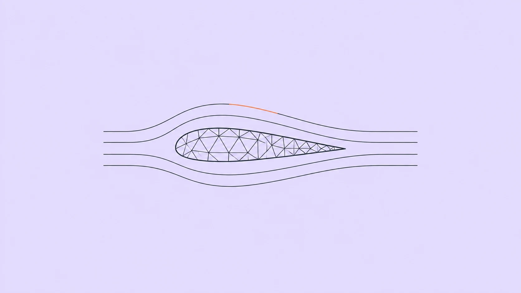
HPC simulation explained: CPUs, GPUs, and scaling

HPC simulation uses high-performance computing to run scientific and engineering models, either by dividing one demanding calculation across processors or by running many independent cases at once. It becomes useful when a workstation cannot fit the model in memory, finish it before a deadline, or process enough variations for the study.

For engineers and researchers choosing infrastructure, the first decision is what needs to scale. One tightly coupled simulation and a batch of independent simulations can need very different systems. This guide explains how to choose CPUs, GPUs, memory, networking, and storage, then test the complete workflow before committing to more capacity.

What high-performance computing adds to simulation

A simulation represents a physical or mathematical system using a model and a numerical method. A solver performs the calculations. HPC supplies resources that can support larger problems, shorter runtimes, or more completed cases, provided the software can use those resources.

There is no fixed number of cores or mesh cells that turns a simulation into HPC. Resource requirements vary with the equations, solver, precision, input size, and stopping criteria. Some demanding work fits on one powerful node; other work needs a coordinated HPC cluster. These HPC systems connect computers so the application can coordinate work across them. Our introduction to high-performance computing covers the broader computing model.

Scientific research combines computation with other evidence. Lawrence Livermore National Laboratory's simulation work illustrates how large-scale modeling supports the study of complex systems. More computing capacity does not establish that a model is accurate: assumptions, numerical convergence, input quality, and comparison with observations still matter.

Why a more detailed model needs more computational work

High performance computing systems are useful when the chosen numerical method creates more work than the available machine can complete. A finer mesh may resolve features that a coarse model misses, while additional time steps, physical effects, or design parameters can increase the calculation further. Higher fidelity simulations still require evidence that the added detail improves the answer.

In engineering applications, simulation can help compare designs before building every physical prototype. An aerospace team might investigate airflow around a component; an energy team might examine a thermal design. These are examples of questions to model, not evidence that simulation replaces physical testing or regulatory validation.

Running simulations also produces work outside the solver. Large outputs may need filtering, visualization, and data analysis before they become useful. Include those tools and stages in the development process: saving an hour of solver time has less value if result processing still takes a day.

Scale one simulation or run more simulations?

Divide one calculation across processors

Parallel processing lets a solver divide computational work among multiple processors. A solver may split a mesh, grid, or set of particles among processes. Those processes calculate their assigned work and exchange the information needed to continue. Shared-memory threads work within a common memory space; distributed-memory execution commonly uses MPI to communicate between processes. Hybrid applications combine approaches, sometimes with GPU acceleration.

Frequent communication makes a workload tightly coupled. For example, neighboring parts of a fluid model may exchange boundary values during each iteration. Making each part smaller eventually leaves less computation between exchanges, so adding processors can produce diminishing returns or even slow the run.

Strong scaling means keeping the total problem fixed while adding resources to reduce elapsed time. Weak scaling increases the total problem with the resources, keeping work per processor roughly fixed. The LLNL parallel-computing tutorial explains these distinct tests. A good weak-scaling result does not establish that the same small model will finish faster on more nodes.

Run independent cases concurrently

Parameter sweeps, sensitivity studies, design-space exploration, and many Monte Carlo workflows involve independent tasks. Each case may use several cores or a GPU, but usually needs little communication with the other cases during its calculation.

Consider an illustrative study with 100 independent design variants. If each variant fits on one instance, assigning separate variants to available instances can increase throughput without dividing any individual solver run across machines. Shared input downloads, licenses, and result collection can still become bottlenecks.

Choose the measurement that matches the project. A single deadline-critical case needs a shorter time to solution. A campaign needs enough validated cases completed within its time and cost limits. Using every available processor for one case may reduce the number of cases completed overall.

Common HPC simulation workloads

Computational fluid dynamics (CFD) models fluid flow and related behavior, such as heat transfer or aerodynamics. The mesh, physical models, solver, and time-stepping method affect memory use and parallel performance.

Finite element analysis (FEA) supports structural, thermal, and other engineering simulations. An explicit transient calculation and an implicit solve can have different communication, memory, and licensing constraints even when they describe the same component.

Molecular dynamics follows the evolution of interacting particles. GPU support depends on the code and the operations used. The GROMACS performance guide, for example, discusses CPU/GPU work distribution, communication overhead, and measurements from the simulation log.

Weather models, electromagnetic solvers, seismic calculations, and reservoir models create other HPC workloads. Their labels do not determine the hardware configuration. A small prototype, a production case, and an ensemble of cases can have different requirements within the same discipline.

Choose CPUs or GPUs from the solver requirements

When CPU execution makes sense

Start with the application's supported execution modes. CPU resources may be the practical choice when the solver lacks a suitable GPU implementation, substantial work remains serial, the model requires more memory than the available GPU configuration can provide, or the supported software and licenses favor CPU execution.

Compare per-core performance, memory bandwidth, and available RAM alongside core count. A solver that spends time waiting for memory or running a serial phase may gain little from additional CPU cores. Establish a working baseline before changing the number of processes or threads.

When GPU acceleration is useful

A GPU can accelerate supported numerical kernels with enough parallel work. It does not automatically accelerate the entire simulation. Check the exact solver version, enabled physical models, precision requirements, GPU architecture, and available GPU memory.

Ansys documents several parallel execution methods and explains how nonparallel work limits total speedup. Treat a vendor benchmark as evidence for its stated configuration, rather than a forecast for a different model.

Consumer and data-center GPUs also differ in characteristics relevant to simulation. Check support for the required numerical precision and the vendor's supported-hardware list. An AI throughput figure alone is not enough to choose a GPU for a scientific solver.

Test multiple GPUs separately

Multiple GPUs help only if the application supports distributing the work effectively. Data exchange, synchronization, and CPU-side work can limit the gain. GPU memory is not automatically available as one pooled address space simply because several devices are installed.

Start with a representative single-GPU run when the problem fits. Test an additional supported configuration and compare elapsed time, memory use, output validity, and cost. If the model needs more than one GPU to fit, use the smallest feasible configuration as the baseline and document that choice.

When a simulation needs multiple nodes

Multiple nodes can provide additional memory and compute capacity. For a tightly coupled solver, they also introduce a network path into the calculation. Latency, bandwidth, communication libraries, placement, and topology can determine whether the extra capacity is useful.

The AWS guidance for tightly coupled workloads treats compute, networking, storage, and deployment as related choices. A collection of cloud instances does not become an efficient HPC cluster just because the solver starts successfully on all of them.

Before a multi-node test, confirm compatible software on every node, the supported MPI configuration, access between nodes, resource allocation, and the required file access. Measure the actual communication-heavy phases. A successful independent batch test does not verify tightly coupled MPI performance.

Failure handling matters as the job grows. Determine whether a failed process or node stops the whole calculation, how the solver saves checkpoints, and whether a restart can recover a useful state. Test recovery before relying on it for an expensive run.

Memory and storage can set the limit

Estimate peak memory from a representative case, including solver workspaces and temporary arrays. Mesh size alone is an unreliable universal sizing rule. Precision, state variables, numerical method, and partitioning affect both host RAM and GPU memory. Leave appropriate headroom and watch peak use during demanding phases.

Plan separately for input data, working files, checkpoints, post-processing, and retained results. Local NVMe can serve a job's scratch space. Shared storage may be needed when processes or stages must access the same files. A parallel file system becomes useful when its shared I/O capability meets a measured requirement; it is not mandatory for every HPC simulation.

Our guide to HPC file systems and parallel storage explains those choices in detail. Object storage can hold inputs and retained outputs, with data staged into the execution environment where necessary. It does not provide the same interface as a mounted POSIX file system.

Checkpoint frequency is a trade-off between write overhead and work lost after failure. Record the time spent writing, check available capacity, and verify that recovery copies survive the failure you are planning for. A checkpoint kept only on storage that disappears with the instance cannot recover an instance loss.

Job management and reliability in simulation workflows

A typical run starts with geometry, a physical system, or another mathematical model. The team prepares a mesh or input dataset, sets solver parameters, stages the data, runs the calculation, saves useful intermediate state, and post-processes the results. Changes to the design or model then create another run.

Save the solver version, dependency versions, input identity, numerical settings, and resource configuration with each result. Reproducible environments help compare hardware fairly and diagnose failures. They do not replace backups of inputs and outputs.

Slurm allocates resources and schedules jobs in many HPC environments. Its job arrays provide a way to manage collections of similar batch jobs. A scheduler coordinates execution; it does not make a serial solver parallel.

Cloud workflows may use a batch service, workflow manager, or scripts. Check what the platform actually automates. Instance lifecycle operations, solver submission, license checks, retries, output validation, and cleanup are separate responsibilities. Make retries distinguish completed work from partial output so a failed transfer does not silently become a successful result.

Software licensing belongs in the capacity plan

Commercial simulation software may license features, parallel resources, or concurrent jobs separately. Check the terms for the exact product and deployment: permitted cloud use, supported core or GPU counts, concurrent capacity, and access to any license server.

The Ansys licensing guide documents product-specific HPC and concurrent-variation options. Avoid applying one product's allowance to every solver. Confirm the current terms with the software provider before renting resources that the license will not let you use.

Include these costs in comparisons. A faster configuration may reduce compute time while increasing the required software entitlement. A large batch may be limited by concurrent licenses before it exhausts available machines.

Cloud or on-premises HPC for simulation?

Cloud infrastructure can be useful for intermittent projects, temporary demand peaks, testing a different configuration, or a study that exceeds a workstation's memory. Availability, quotas, setup time, data transfer, and software support still constrain the work. Cloud capacity should not be treated as unlimited.

An existing on-premises system may be a good fit for steady utilization, specialized interconnects, stable software requirements, or large datasets that already reside nearby. Include hardware, operations, maintenance, and waiting time in the comparison instead of comparing a rental rate with purchase price alone.

Before moving confidential research data, check access controls, software security responsibilities, and the approved location for the data. Technical compatibility alone does not settle those requirements.

A hybrid approach needs a clear data and software plan. Decide which cases can move, how their inputs and results will be transferred, and how licenses and configuration remain consistent. Start with a representative workload whose success criteria are clear.

How to benchmark an HPC simulation

Use a case that represents the expected model size and physical behavior. Keep the solver version, convergence targets, precision, and outputs comparable. A faster run with different stopping criteria is not a fair infrastructure comparison.

• Time to solution: record solver time and the end-to-end time needed for a usable result, including staging and post-processing. Track queue and setup time separately.
• Throughput: count completed, valid cases within the relevant time window.
• Scaling: compare runtime as resources change while recording whether the problem size stays fixed or grows.
• Resource use: measure peak memory, CPU/GPU utilization, communication waits, and I/O delays.
• Total cost: include compute, storage, transfers, licenses, failed runs, and operating work.

For a simple hypothetical example, a fixed case taking 10 hours on one node and 6 hours on two has a speedup of about 1.67 and parallel efficiency of about 83%. It uses 12 node-hours instead of 10. At the same hourly price per node, the solver run costs 20% more in compute while finishing 4 hours earlier. Whether that trade-off is worthwhile depends on the deadline and the full workflow.

Repeat tests to understand variation. Check that results satisfy the application's validation criteria, and record the configuration that produced them. Do not assume bit-for-bit identical output is the only valid comparison when execution order or numerical libraries change; use a scientifically appropriate comparison method.

Which simulation workloads could fit Hivenet's Compute?

Hivenet's Compute provides CPU and GPU instance options for software that fits the selected environment. Potential uses include single-node simulations, supported GPU solvers, independent parameter studies, and pre- or post-processing. These are workloads to evaluate, not claims that every solver is supported or included.

The Compute FAQ documents container and virtual-machine runtimes, SSH access, and local NVMe storage. Choose the runtime and current configuration around the application, then test a real case. Keep retained inputs and results in storage with the lifecycle and recovery properties the project needs.

For tightly coupled multi-node work, confirm the proposed networking, MPI support, storage interface, scheduling, and support arrangements with Hivenet before committing. Renting instances alone does not establish a managed Slurm cluster, a parallel file system, or a particular interconnect performance level.

Start with one supported case, validate its results, and measure time and cost. Expand to more resources or concurrent jobs only when that evidence supports the next step.

Frequently asked questions

Does every simulation need HPC?

No. A workstation may be sufficient for smaller models and early development. HPC becomes useful when memory, runtime, or the number of required cases exceeds the capacity available locally.

Is HPC simulation the same as GPU computing?

No. HPC simulation can use CPUs, GPUs, or a combination. GPU acceleration depends on the solver's implementation and the parts of the calculation that it supports.

Will more cores always finish a simulation faster?

No. Serial work, communication, memory access, and I/O can limit or reverse the gain. Test the same case on a few feasible configurations and choose from measured results.

Is HPC the same as AI?

No. HPC describes computing methods and infrastructure; AI describes a class of methods and applications. Machine learning may support a simulation workflow, for example through a surrogate model or result analysis, but it introduces its own training and validation requirements.